How to Build a Waste Classifier: A Case Study from ML Zoomcamp

How does ML Zoomcamp turn course content into practical ML engineering? In this case study, Serena Haidar walks through her final project from ML Zoomcamp: training an Xception-based image classifier on ~15,000 waste images, reaching 93.3% test accuracy, and serving predictions via a Flask API packaged in Docker.

If you’re evaluating this free course, this article shows how a graduate moves from a notebook to a small production app—what gets built, why each step matters, and how to approach the work methodically.

At DataTalks.Club, ML Zoomcamp is a free, four-month online course on core machine learning and taking models to production. To complete the course and earn a certificate, students deliver an end-to-end final project that turns course concepts into a working system.

Interview with Serena about Her Project Idea

Q: How did you select the problem for your final project?

The idea behind my project was to accurately classify waste, ensuring that different types of waste are sent to the appropriate locations.

For example, plastics, metals, and glass should go to recycling centers. When they end up in regular trash bins, they can remain for decades, contaminating soil and harming wildlife. Organic waste like food scraps, on the other hand, should be composted. If it ends up in landfills instead, it breaks down without oxygen and releases methane, a greenhouse gas many times more potent than carbon dioxide.

These two sorting mistakes can speed up environmental damage and worsen climate change.

Q: How did you technically approach it?

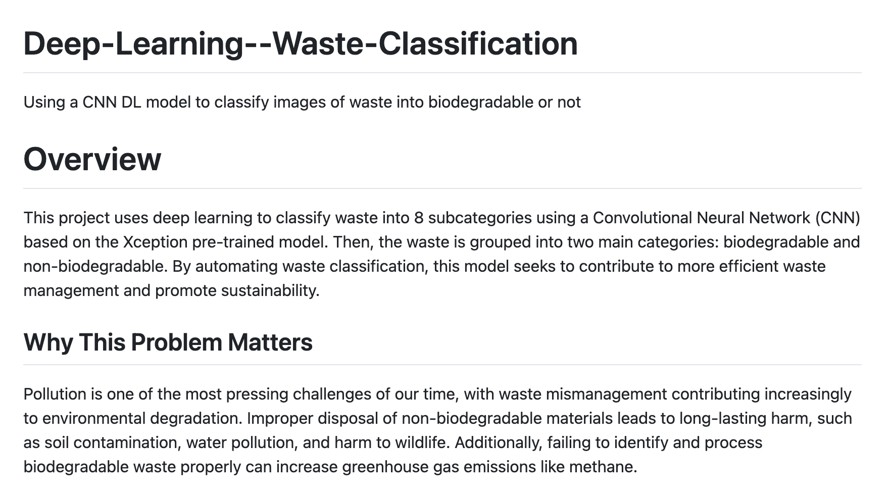
The initial task was to differentiate between biodegradable and non-biodegradable waste, then classify it further into 8 subcategories: e-waste, food waste, leaf waste, metal waste, paper waste, plastic bags, plastic bottles, and wood waste.

For classification into subcategories, I chose to use deep learning, specifically a Convolutional Neural Network (CNN) based on the Xception pre-trained model. To consider the project successful, the benchmarks included: an accuracy score of over 90% and a small model size suitable for lightweight deployment.

Q: Who could potentially use a similar approach to waste classification in real-life settings?

This project helps companies begin automating sustainable waste management. It’s the very first link in a chain of actions that lead to improved recycling.

Here’s how the process works:

• An embedded camera (for example, an ESP32‑CAM) monitors each piece of waste as it arrives.
• The device runs a simple image classification model to determine whether the item is plastic, metal, glass, organic, etc.
• It sends that label to the sorting equipment downstream.

Correct labels lead to fewer mistakes, less manual checking, and quicker routing of materials to recycling or composting.

Technical Overview

In this section, Serena will guide you through the key components of her project.

Data Selection

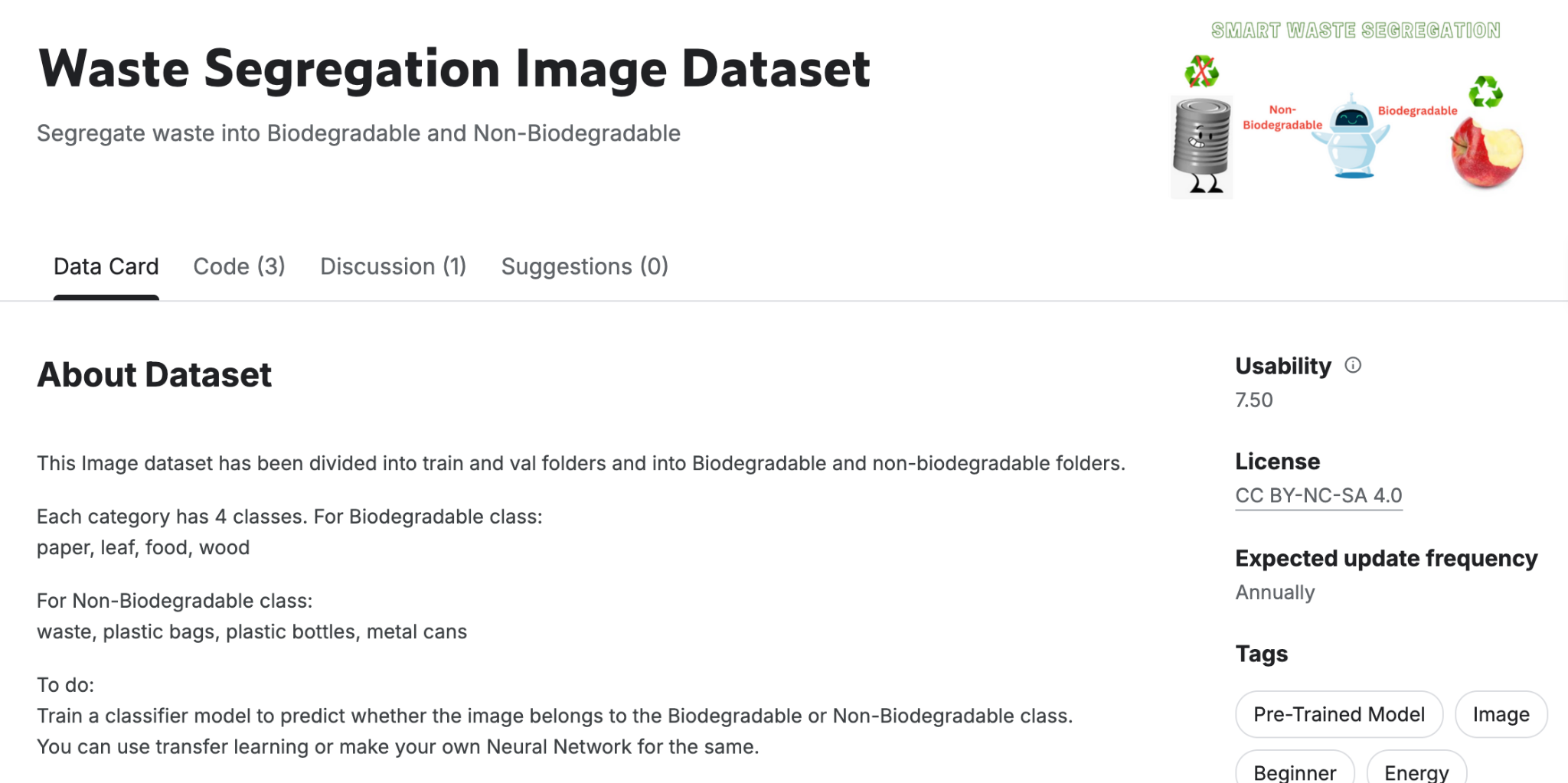
I used a public dataset from Kaggle, comprising 15,200 images, split into 3 subsets: train, test, and validation.

Each subset contains images for 8 classes:

• Train: 13,999 images
• Validation: 1,201 images
• Test: 1,201 images

Images were resized to 150x150 initially to reduce training time and later to 299x299 for final training.

Model Selection

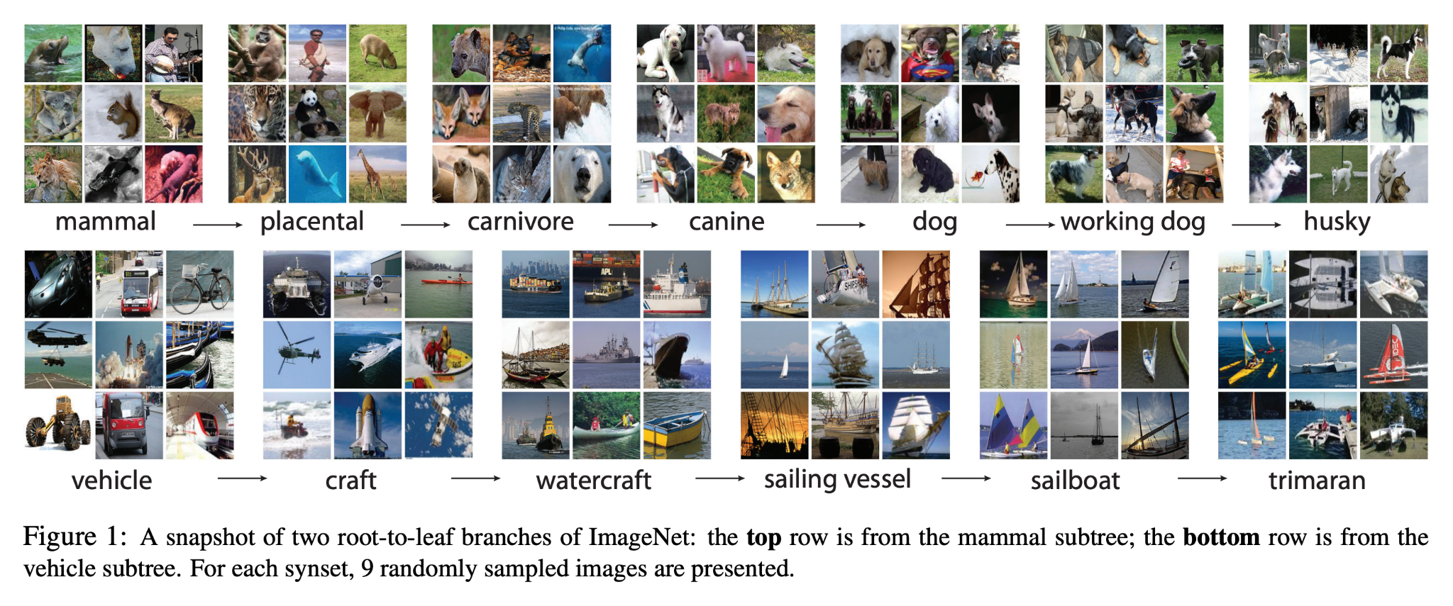
Instead of training a model from scratch, I used a pre-trained Keras model from the official website. After comparing models based on performance and size, I chose the Xception model. It’s a CNN architecture trained on over a million ImageNet images with 1000 output classes.

Xception Model Architecture

The Xception model consists of a series of convolutional layers arranged into a deep CNN architecture. It starts with two standard convolution layers, followed by 36 depthwise separable convolution layers organized into 14 modules.

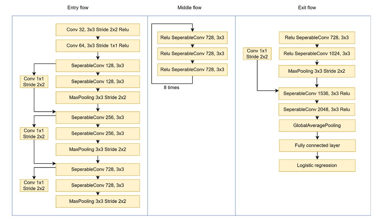
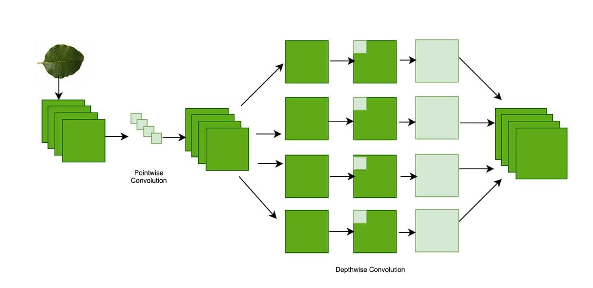
Each module contains a stack of operations like depthwise convolutions (which filter each input channel separately) and pointwise convolutions (which combine the outputs), allowing the model to be both efficient and powerful.

These layers are designed to extract increasingly abstract features from input images, starting with basic edges and colors in early layers and progressing to complex textures and shapes in deeper layers. The architecture concludes with a Global Average Pooling layer and a fully connected Dense layer of 1000 neurons with a softmax activation, used to classify images into 1000 categories from the ImageNet dataset.

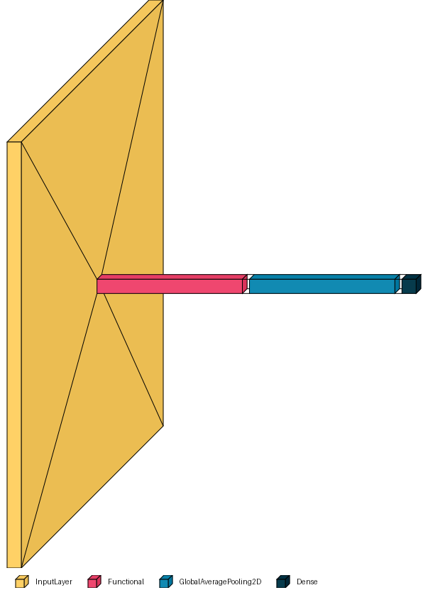
You can visualize the block diagram of the Xception model by running this code:

model = Xception(weights=’imagenet’, input_shape=(299, 299, 3))

visualkeras.layered_view(model, legend=True)

</figure>

My Modifications of the Original Model

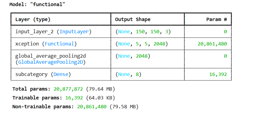
For the waste classification task, I removed the top layer and added a new custom head to predict 8 waste classes. The “top layer” in a pre-trained model is the final Dense (fully connected) layer that maps extracted features into the original classes. In the case of Xception, the top layer maps to the original 1000 classes from the ImageNet dataset.

Since my dataset only contains 8 categories of waste, I replaced this layer with a custom classification head to output probabilities for only these 8 classes. This technique is known as “transfer learning,” where we retain the convolutional layers of the Xception model, remove the top (dense) layer, and add a new one to learn our specific classes and make predictions.

Transfer learning helps reduce training time and improves performance by leveraging features learned from a large dataset, such as ImageNet.

Specifically, I used:

• A dense layer for the 8 subcategories.
• Another dense layer for biodegradability.

After adding a new top layer, we can visualize the model summary using model.summary().

Hyperparameter Tuning

The first model didn’t perform well enough. The validation accuracy was oscillating between 0.83 and 0.88. Hyperparameter tuning was necessary.

I determined the optimal learning rate by training the model on four different learning rates: [0.0001, 0.001, 0.01, 0.1]. After plotting, I chose lr=0.001 as the best value, as it achieved the highest validation accuracy.

Then, I added Dropout for regularization, a technique that randomly deactivates a small number of neurons during training, changing which neurons are active between each epoch. It helps prevent overfitting and encourages the network to learn more robust features.

Finally, I used softmax activation with 8 units as the output layer of my model. This setup allows the model to output a probability for each of the 8 waste subcategories. Softmax is ideal for the output layer of a multi-class classification network because it assigns a probability score to each class that sums up to 1.

Training Strategy and Optimization

In addition to tuning the learning rate and adding dropout, I implemented a few more strategies to improve performance and stability during training:

• Checkpointing: It’s a technique that saves the best-performing model from a list of training models based on a specific parameter. In my project, I used ModelCheckpoint callback from keras.callbacks to automatically save only the best version of the model (the one with the highest validation accuracy). This ensured that training didn’t overwrite a good model with a worse one in later epochs.
• Inner Dense Layer Tuning: I experimented with different values for the inner_size (number of units) parameter in the Dense layer before the output. After testing 3 values: [10, 100, 500], I found that 100 worked best. This layer acts as the bridge between the extracted features and the final classification layer.

Data augmentation

To enrich the dataset, instead of taking pictures of new images, we can apply a technique called data augmentation.

This adds images to the dataset from the existing images, by applying augmentations to the images, such as:

• flip (horizontally or vertically)
• rotate (by an angle, clockwise or counter-clockwise)
• shift (by height or width)
• shear (extend from one corner)
• zoom (in/out, horizontally/vertically)
• brightness or contrast shifts

This technique helps with overfitting by increasing data diversity.

After data augmentation, I trained a larger model with 299x299 images, which is closer to the production environment where users will upload photos and receive classification results for their waste.

Final results

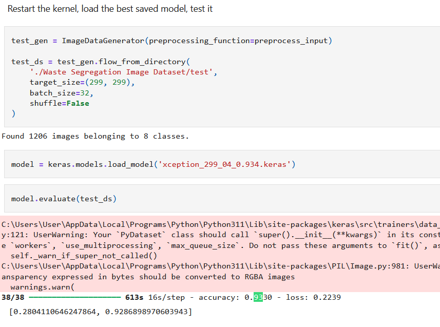
After tuning many hyperparameters and training the model on larger images, I tested it on the test data subset to evaluate its performance. Since the best model is saved using callbacks, we restart the kernel, load the best saved model, and then test it.

model = keras.models.load_model(‘xception_299_04_0.934.keras’)

model.evaluate(test_ds)

The final accuracy is 93.3%, which is above our threshold.

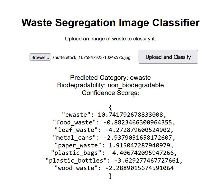
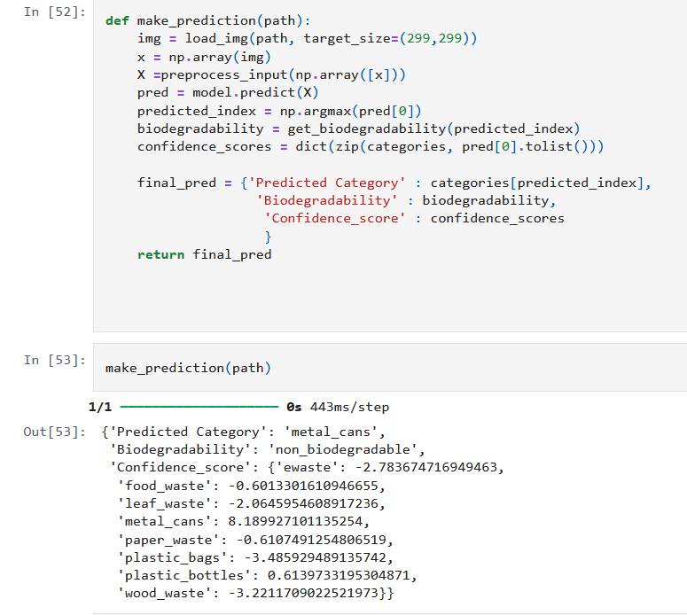
Then, we can test it on a random image of a metal can that it hasn’t seen before from the val dataset, and get the final prediction, which features the predicted category, biodegradability, and confidence scores.

Serving and Deployment

To deploy my model and create a user-friendly interface that allows users to upload an image and receive a prediction, I took the following steps.

Step 1: Built a Flask API for inference

I created a Flask web server that receives image uploads, passes them to the model, and returns the prediction. This allows the model to serve predictions through HTTP requests.

Step 2: Dockerized the app for consistent deployment

To ensure the app runs identically across different environments, I created a Docker container containing the Flask app, the trained model, and all necessary dependencies.

Docker usage:

docker build -t waste-segregation-app .

This command builds the Docker image from the Dockerfile and names it waste-segregation-app

docker run -p 9696:9696 waste-segregation-app

This runs the container and maps port 9696 on your machine to the container’s port 9696, making the API accessible

Step 3: Inference

As a result, a user can call the model and retrieve results using either a command line or a web interface.

Option 1: Using the command line

curl -X POST -F “file=@your_image.jpg” http://localhost:9696/predict

This sends a POST request with an image to the /predict endpoint, and the model returns the predicted waste category

Option 2: Using the web interface

I created a simple HTML web interface where a user can upload an image, click a button, and receive a classification result. This interface is connected to the same backend. At localhost:9696

</figure>

Screenshot of the web interface and the result after uploading an image from the Internet.